Function Plotting

The plotting tool lets you create interactive 2D and 3D graphs inside a Drawing Area. You can plot functions, inequalities, parametric curves, vector fields, and more — all with a visual editor.

Opening the Plot Editor

Click the plot icon in the Drawing Area toolbar to open the plot settings dialog.

The dialog has four tabs: Expressions, Axes, X Axis, and Y Axis. A live preview of the graph is shown on the right side.

Expressions

The Expressions tab is where you add and configure the functions to plot.

Adding an Expression

Click + Add to see all available expression types:

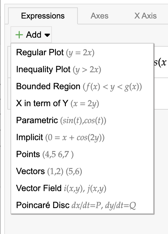
Type	Format	Description
Regular Plot	y = 2x	Standard function of x
Inequality Plot	y > 2x	Shade the region above or below a function
Bounded Region	f(x) < y < g(x)	Shade the region between two functions
X in term of Y	x = 2y	Function where x is expressed in terms of y
Parametric	sin(t), cos(t)	Parametric curve defined by x(t) and y(t)
Implicit	0 = x + cos(2y)	Implicit equation in x and y
Points	4,5 6,7	Plot individual points
Vectors	(1,2) (5,6)	Draw arrow vectors
Vector Field	i(x,y), j(x,y)	Visualize a 2D vector field
Poincaré Disc	dx/dt=P, dy/dt=Q	Phase portrait of a dynamical system

Expression Editor

Each expression has an inline math editor where you type the function. Below the expression you can configure:

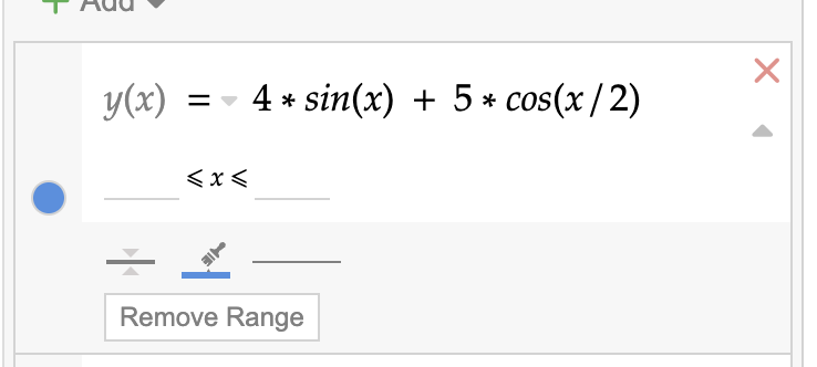
• Color — click the color circle to change the plot color
• Range — optionally restrict the domain (e.g., limit x to a specific interval)
• Line style — choose between solid, dashed, or other stroke types
• Line thickness — adjust the stroke width
• Remove Range — remove the domain restriction

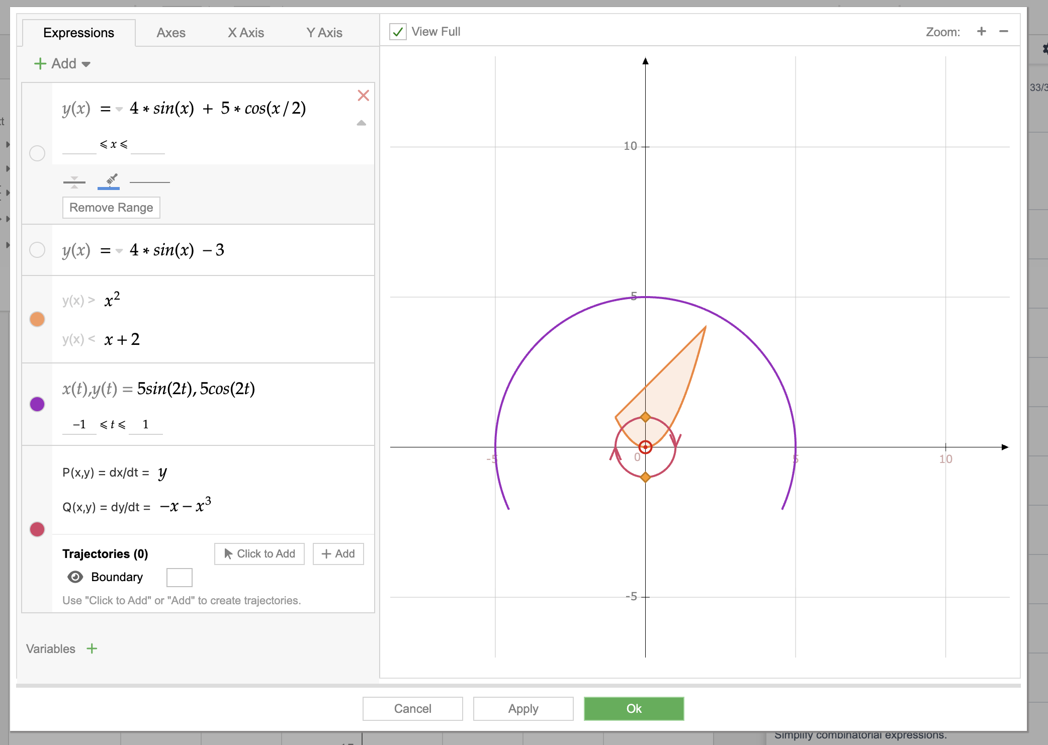
Multiple Expressions

You can add multiple expressions of different types to the same graph. Each expression gets its own color and is plotted together on the same axes:

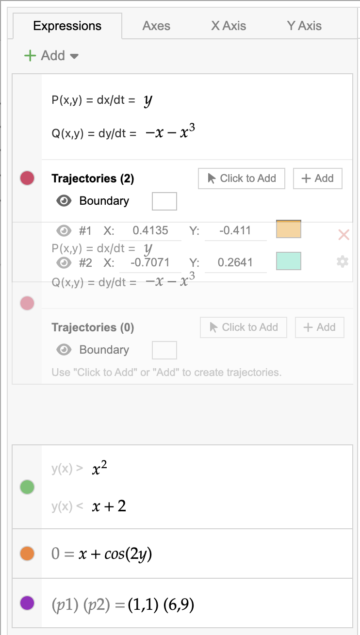
Rearranging Expressions

You can drag and drop expressions to reorder them in the list. The order affects the drawing order — expressions lower in the list are drawn on top of earlier ones.

Show / Hide Expressions

Click the visibility toggle (the colored circle) next to an expression to hide it from the graph without deleting it. This is useful for temporarily removing a plot from view while keeping its configuration. Click again to show it.

Variables

At the bottom of the Expressions tab, click Variables + to define named variables (single letters a–z) with numeric values. These variables can be referenced inside your expressions, making it easy to adjust parameters without editing the function.

Axes

The Axes tab controls the overall appearance of the coordinate system.

Axes Type

Three visual styles are available:

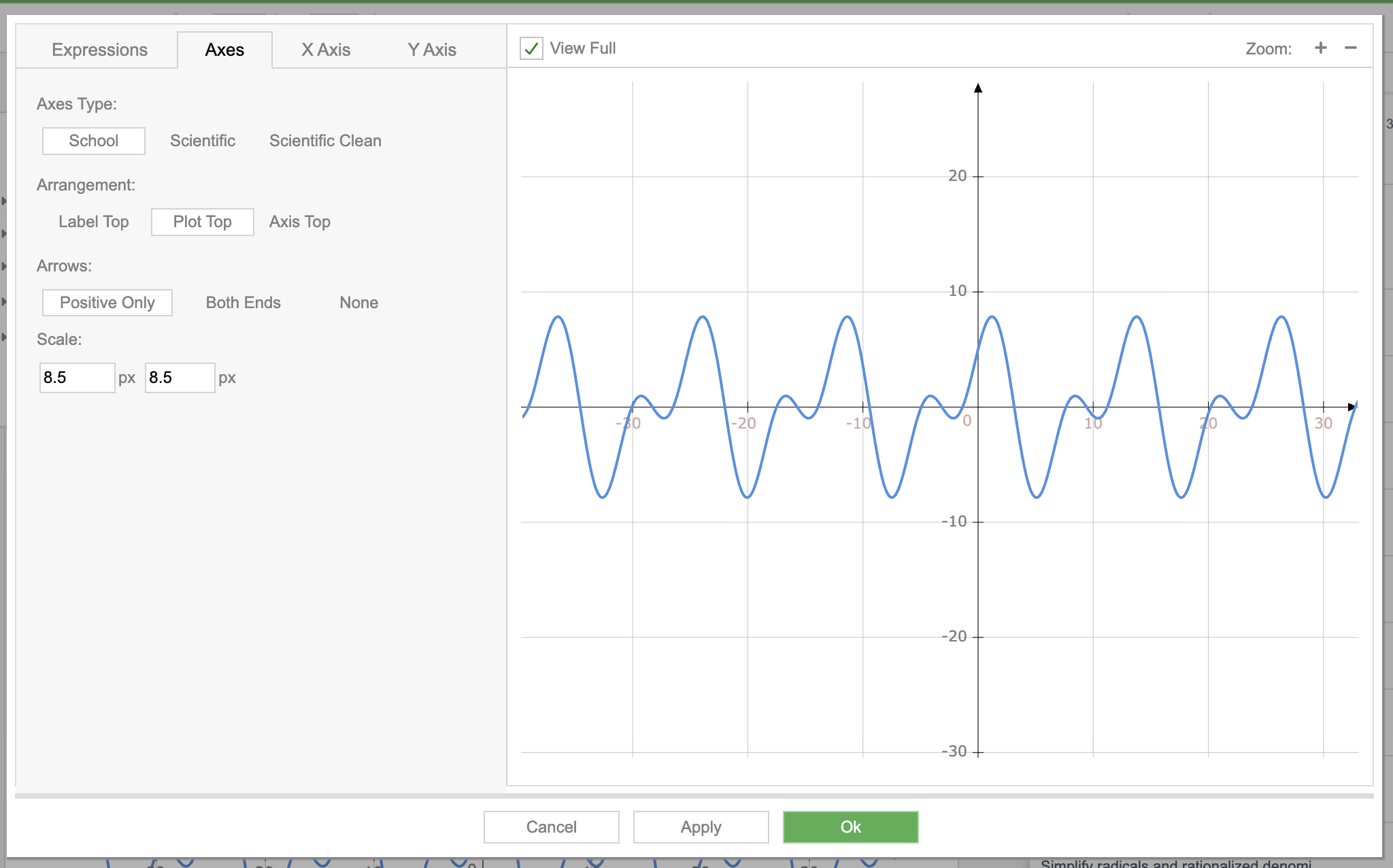
School — traditional style with axis labels and arrows:

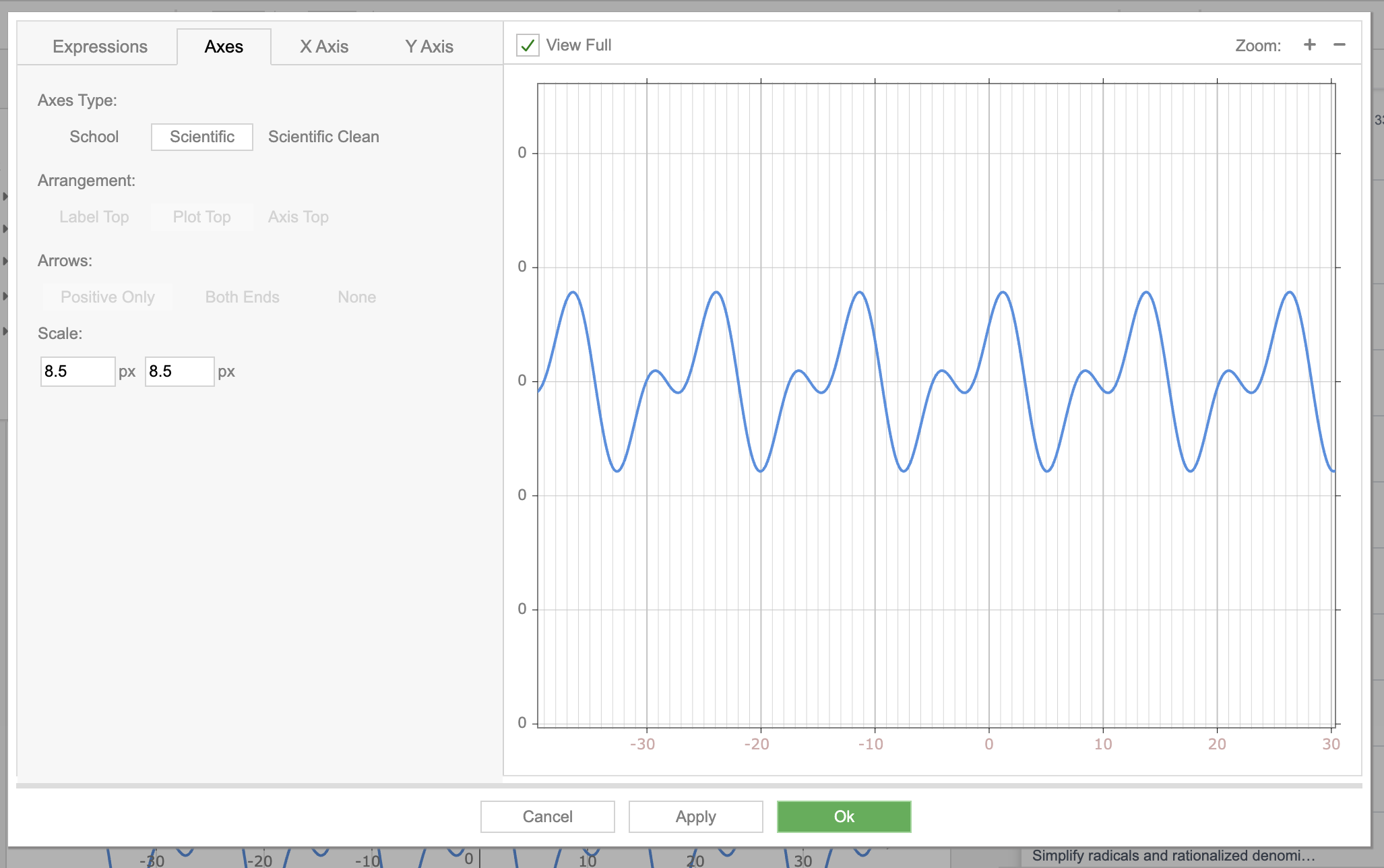
Scientific — grid-based with labeled tick marks and no arrows:

Scientific Clean — minimal grid with no axis lines.

Arrangement (School only)

Controls the layering order of axis, plot, and labels:

Option	Description
Label Top	Labels drawn on top of everything
Plot Top	Plot curves drawn on top of axes
Axis Top	Axis lines drawn on top of plots

Arrows (School only)

Option	Description
Positive Only	Arrows at the positive end of each axis
Both Ends	Arrows at both ends of each axis
None	No arrows on axes

Scale

Set the scale in pixels for each axis independently. The default is 8.5 px per unit for both X and Y.

X Axis / Y Axis

The X Axis and Y Axis tabs configure individual axis properties. Both tabs have the same options:

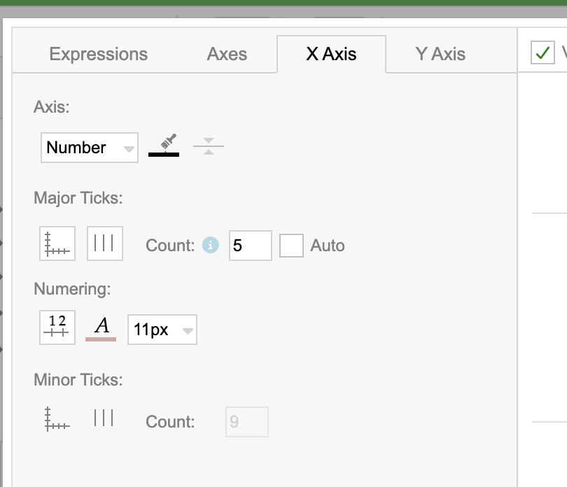
Axis Type

• Number — standard numeric labels (1, 2, 3, …)
• Radian — labels in multiples of π

Major Ticks

• Show axis — toggle the tick marks on or off
• Grid — toggle vertical/horizontal grid lines
• Count — number of major tick divisions (or Auto)

Numbering

• Show numbers — toggle numeric labels on ticks
• Text color — color picker for the labels
• Font size — label font size (8–22 px)

Minor Ticks

• Show axis — toggle minor tick marks
• Grid — toggle minor grid lines
• Count — number of minor divisions between major ticks

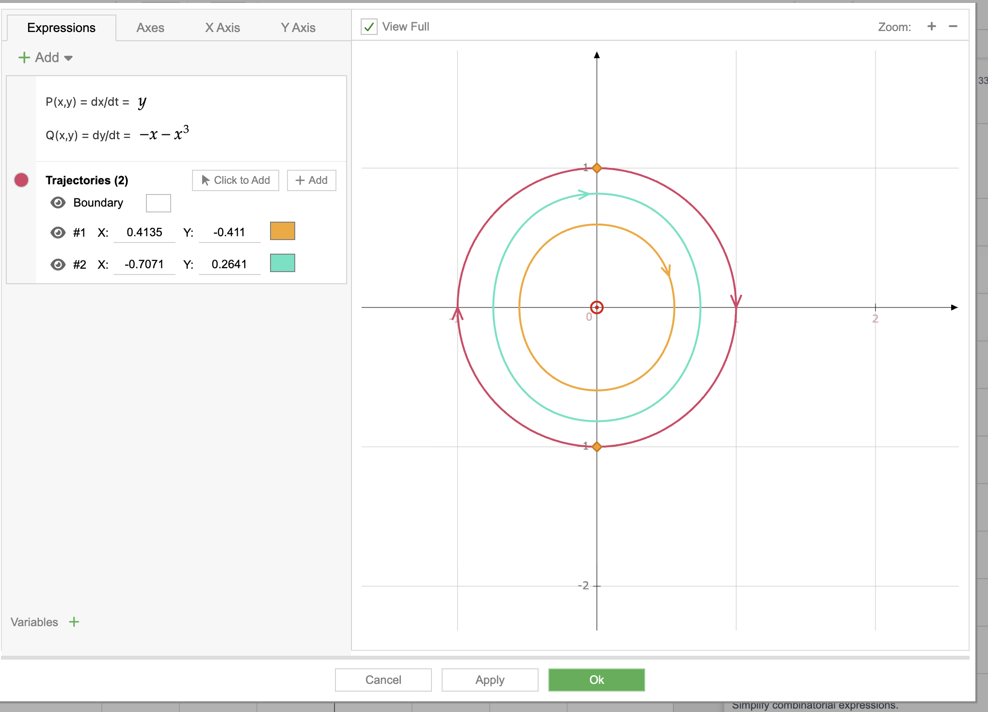
Poincaré Disc

The Poincaré Disc expression type plots a phase portrait of a 2D dynamical system defined by:

• P(x,y) = dx/dt — the x-component of the vector field
• Q(x,y) = dy/dt — the y-component of the vector field

Trajectories

Trajectories show the flow of the system from given initial conditions:

• Click to Add — click directly on the plot to place a trajectory starting point
• + Add — manually enter the initial (x, y) coordinates
• Each trajectory has its own color and visibility toggle
• The Boundary circle shows the boundary of the Poincaré disc

Buttons

At the bottom of the dialog:

• Cancel — discard changes and close
• Apply — apply changes without closing (useful for previewing)
• Ok — apply changes and close the dialog

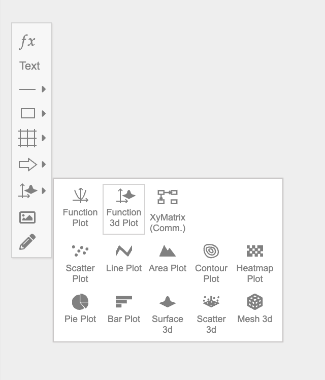
3D Plotting

Mathcha also supports 3D plotting. To create a 3D plot, select Function 3d Plot from the Drawing Area toolbar:

3D Expression Types

Click + Add in the 3D plot editor to see the available expression types:

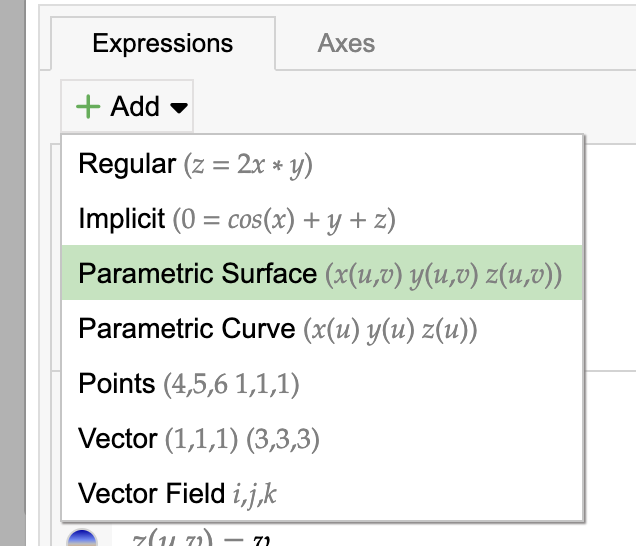
Type	Format	Description
Regular	z = 2x * y	Surface defined as z in terms of x and y
Implicit	0 = cos(x) + y + z	Implicit 3D equation
Parametric Surface	x(u,v), y(u,v), z(u,v)	Surface defined by parametric equations in two parameters
Parametric Curve	x(u), y(u), z(u)	Space curve defined by parametric equations in one parameter
Points	4,5,6 1,1,1	Plot individual 3D points
Vector	(1,1,1) (3,3,3)	Draw 3D arrow vectors
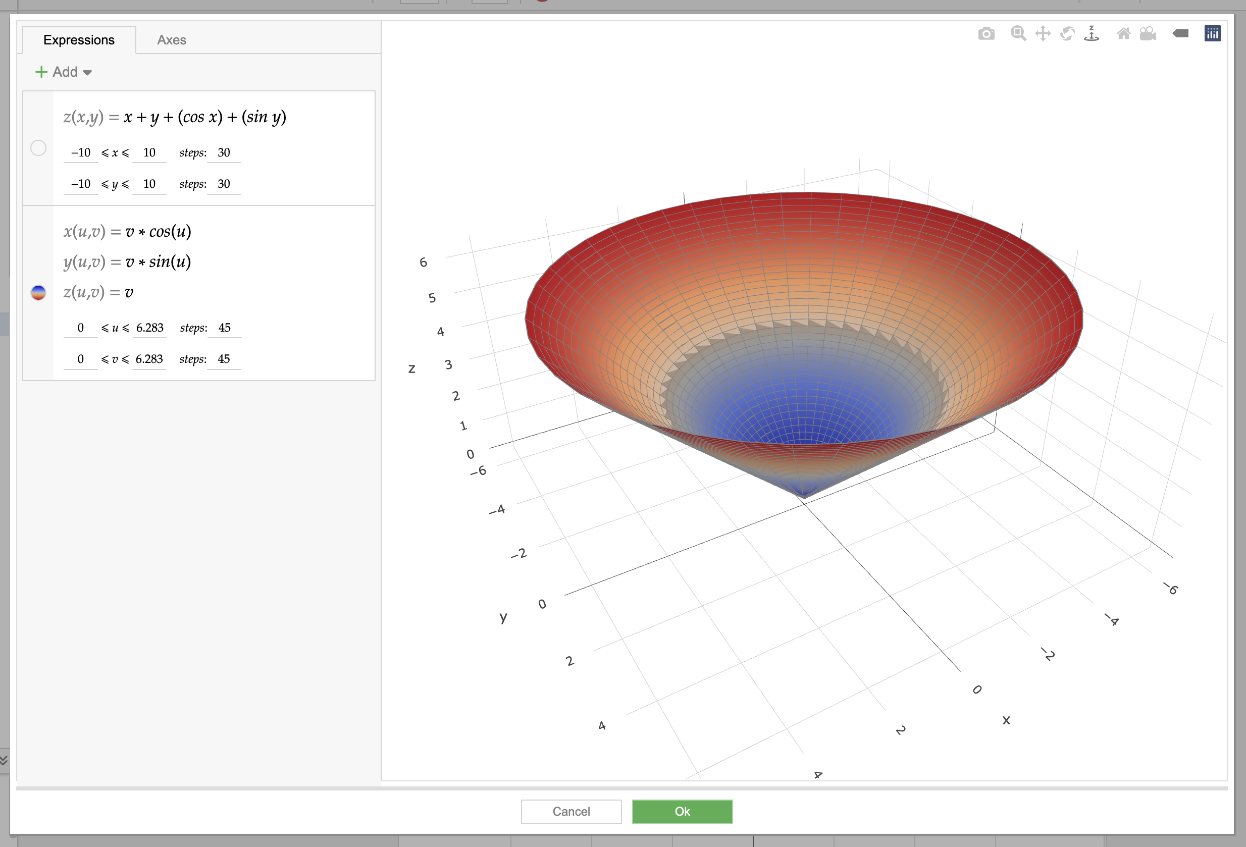
Vector Field	i,j,k	Visualize a 3D vector field

Example: Drawing a Cone with Parametric Surface

You can create complex 3D shapes using the Parametric Surface type. For example, a circular cone can be expressed as:

• x(u,v) = v * cos(u)
• y(u,v) = v * sin(u)
• z(u,v) = v

With u range [0, 2π] and v range [0, h] (where h is the desired height).

Other approaches for plotting cone-like surfaces:

• Regular surface: z = sqrt(x² + y²) for an upward cone, with appropriate x/y ranges
• Implicit surface: x² + y² - z² = 0